Joining Data

Code for Quiz 6, more dplyr and our first interactive chart using echarts4r.

Steps 1-6.

1. Load the R packages we will use.

library(tidyverse)
library(echarts4r)
library(hrbrthemes)

2. Read the data in the files, drug_cos.csv, health_cos.csv into R and assign to the variables drug_cos and health_cos, respectively

drug_cos  <- read_csv("https://estanny.com/static/week6/drug_cos.csv")

health_cos  <- read_csv("https://estanny.com/static/week6/health_cos.csv")

3. Use glimpse to get a glimpse of the data.

drug_cos %>% glimpse()

Rows: 104
Columns: 9
$ ticker       <chr> "ZTS", "ZTS", "ZTS", "ZTS", "ZTS", "ZTS", "ZTS…
$ name         <chr> "Zoetis Inc", "Zoetis Inc", "Zoetis Inc", "Zoe…
$ location     <chr> "New Jersey; U.S.A", "New Jersey; U.S.A", "New…
$ ebitdamargin <dbl> 0.149, 0.217, 0.222, 0.238, 0.182, 0.335, 0.36…
$ grossmargin  <dbl> 0.610, 0.640, 0.634, 0.641, 0.635, 0.659, 0.66…
$ netmargin    <dbl> 0.058, 0.101, 0.111, 0.122, 0.071, 0.168, 0.16…
$ ros          <dbl> 0.101, 0.171, 0.176, 0.195, 0.140, 0.286, 0.32…
$ roe          <dbl> 0.069, 0.113, 0.612, 0.465, 0.285, 0.587, 0.48…
$ year         <dbl> 2011, 2012, 2013, 2014, 2015, 2016, 2017, 2018…

health_cos %>% glimpse()

Rows: 464
Columns: 11
$ ticker      <chr> "ZTS", "ZTS", "ZTS", "ZTS", "ZTS", "ZTS", "ZTS"…
$ name        <chr> "Zoetis Inc", "Zoetis Inc", "Zoetis Inc", "Zoet…
$ revenue     <dbl> 4233000000, 4336000000, 4561000000, 4785000000,…
$ gp          <dbl> 2581000000, 2773000000, 2892000000, 3068000000,…
$ rnd         <dbl> 427000000, 409000000, 399000000, 396000000, 364…
$ netincome   <dbl> 245000000, 436000000, 504000000, 583000000, 339…
$ assets      <dbl> 5711000000, 6262000000, 6558000000, 6588000000,…
$ liabilities <dbl> 1975000000, 2221000000, 5596000000, 5251000000,…
$ marketcap   <dbl> NA, NA, 16345223371, 21572007994, 23860348635, …
$ year        <dbl> 2011, 2012, 2013, 2014, 2015, 2016, 2017, 2018,…
$ industry    <chr> "Drug Manufacturers - Specialty & Generic", "Dr…

4. Which variables are the same in both data sets?

names_drug  <- drug_cos %>% names()
names_health  <- health_cos %>% names()
intersect(names_drug, names_health)

[1] "ticker" "name"   "year"  

5. Select subset of variables to work with

• For drug_cos select(in this order): ticker, year, grossmargin

  • extract observations for 2018
  • assign output to drug_subset

• For health_cos select(in this order): ticker, year, revenue, gp, industry

  • extract observations for 2018
  • assign output to health_subset

drug_subset  <- drug_cos %>% 
  select(ticker, year, grossmargin) %>% 
  filter(year == 2018)

health_subset  <- health_cos %>% 
  select(ticker, year, revenue, gp, industry) %>% 
  filter(year == 2018)

6. Keep all the rows and columns drug_subset join with columns in health_subset

drug_subset %>% left_join(health_subset)

# A tibble: 13 x 6
   ticker  year grossmargin   revenue        gp industry              
   <chr>  <dbl>       <dbl>     <dbl>     <dbl> <chr>                 
 1 ZTS     2018       0.672   5.82e 9   3.91e 9 Drug Manufacturers - …
 2 PRGO    2018       0.387   4.73e 9   1.83e 9 Drug Manufacturers - …
 3 PFE     2018       0.79    5.36e10   4.24e10 Drug Manufacturers - …
 4 MYL     2018       0.35    1.14e10   4.00e 9 Drug Manufacturers - …
 5 MRK     2018       0.681   4.23e10   2.88e10 Drug Manufacturers - …
 6 LLY     2018       0.738   2.46e10   1.81e10 Drug Manufacturers - …
 7 JNJ     2018       0.668   8.16e10   5.45e10 Drug Manufacturers - …
 8 GILD    2018       0.781   2.21e10   1.73e10 Drug Manufacturers - …
 9 BMY     2018       0.71    2.26e10   1.60e10 Drug Manufacturers - …
10 BIIB    2018       0.865   1.35e10   1.16e10 Drug Manufacturers - …
11 AMGN    2018       0.827   2.37e10   1.96e10 Drug Manufacturers - …
12 AGN     2018       0.861   1.58e10   1.36e10 Drug Manufacturers - …
13 ABBV    2018       0.764   3.28e10   2.50e10 Drug Manufacturers - …

Question: join_ticker

• start with drug_cos
• extract observations for the ticker MYL from drug_cos
• assign output to the variable drug_cos_subset

drug_cos_subset  <- drug_cos %>%
  filter(ticker == "MYL")

---

• Display drug_cos_subset

drug_cos_subset

# A tibble: 8 x 9
  ticker name  location ebitdamargin grossmargin netmargin   ros   roe
  <chr>  <chr> <chr>           <dbl>       <dbl>     <dbl> <dbl> <dbl>
1 MYL    Myla… United …        0.245       0.418     0.088 0.161 0.146
2 MYL    Myla… United …        0.244       0.428     0.094 0.163 0.184
3 MYL    Myla… United …        0.228       0.44      0.09  0.153 0.209
4 MYL    Myla… United …        0.242       0.457     0.12  0.169 0.283
5 MYL    Myla… United …        0.243       0.447     0.09  0.133 0.089
6 MYL    Myla… United …        0.19        0.424     0.043 0.052 0.044
7 MYL    Myla… United …        0.272       0.402     0.058 0.121 0.054
8 MYL    Myla… United …        0.258       0.35      0.031 0.074 0.028
# … with 1 more variable: year <dbl>

• use left_join to combine the rows and columns of drug_cos_subset with the columns of health_cos
• assign the output to combo_df

combo_df  <- drug_cos_subset %>% 
  left_join(health_cos)

---

• Display combo_df

combo_df

# A tibble: 8 x 17
  ticker name  location ebitdamargin grossmargin netmargin   ros   roe
  <chr>  <chr> <chr>           <dbl>       <dbl>     <dbl> <dbl> <dbl>
1 MYL    Myla… United …        0.245       0.418     0.088 0.161 0.146
2 MYL    Myla… United …        0.244       0.428     0.094 0.163 0.184
3 MYL    Myla… United …        0.228       0.44      0.09  0.153 0.209
4 MYL    Myla… United …        0.242       0.457     0.12  0.169 0.283
5 MYL    Myla… United …        0.243       0.447     0.09  0.133 0.089
6 MYL    Myla… United …        0.19        0.424     0.043 0.052 0.044
7 MYL    Myla… United …        0.272       0.402     0.058 0.121 0.054
8 MYL    Myla… United …        0.258       0.35      0.031 0.074 0.028
# … with 9 more variables: year <dbl>, revenue <dbl>, gp <dbl>,
#   rnd <dbl>, netincome <dbl>, assets <dbl>, liabilities <dbl>,
#   marketcap <dbl>, industry <chr>

• Note: the variables ticker, name, location, and industry are the same for all the observations.

---

• assign the company name to co_name

co_name  <- combo_df %>% 
  distinct(name) %>% 
  pull()

---

• assign the company location to co_location

co_location  <- combo_df %>% 
  distinct(location) %>% 
  pull()

---

• assign the industry to co_industry group.

co_industry  <- combo_df %>% 
  distinct(industry) %>% 
  pull()

Put the r inline commands used in the blanks below. When you knit the document the results of the commands will be displayed in your text.

The company Mylan NV is located in United Kingdom and is a member of the Drug Manufacturers - Specialty & Generic industry group.

---

• start with combo_df
• select the variables(in this order): year, grossmargin, netmargin, revenue, gp, netincome
• assign the output to combo_df_subset

combo_df_subset  <- combo_df %>% 
  select(year, grossmargin, netmargin, revenue, gp, netincome)

---

• display combo_df_subset

combo_df_subset

# A tibble: 8 x 6
   year grossmargin netmargin     revenue         gp netincome
  <dbl>       <dbl>     <dbl>       <dbl>      <dbl>     <dbl>
1  2011       0.418     0.088  6129825000 2563364000 536810000
2  2012       0.428     0.094  6796100000 2908300000 640900000
3  2013       0.44      0.09   6909100000 3040300000 623700000
4  2014       0.457     0.12   7719600000 3528000000 929400000
5  2015       0.447     0.09   9429300000 4216100000 847600000
6  2016       0.424     0.043 11076900000 4697000000 480000000
7  2017       0.402     0.058 11907700000 4783100000 696000000
8  2018       0.35      0.031 11433900000 4001600000 352500000

---

• create the variable grosmargin_check to compare with the variable grossmargin They should be equal.

  • grossmargin_check = gp / revenue

• create the variable close_enough to check that the absolute value of the difference between grossmargin_check and gross_margin is less than .001

combo_df_subset %>% 
  mutate(grossmargin_check = gp / revenue,
         close_enough = abs(grossmargin_check - grossmargin) < .001)

# A tibble: 8 x 8
   year grossmargin netmargin revenue     gp netincome
  <dbl>       <dbl>     <dbl>   <dbl>  <dbl>     <dbl>
1  2011       0.418     0.088 6.13e 9 2.56e9 536810000
2  2012       0.428     0.094 6.80e 9 2.91e9 640900000
3  2013       0.44      0.09  6.91e 9 3.04e9 623700000
4  2014       0.457     0.12  7.72e 9 3.53e9 929400000
5  2015       0.447     0.09  9.43e 9 4.22e9 847600000
6  2016       0.424     0.043 1.11e10 4.70e9 480000000
7  2017       0.402     0.058 1.19e10 4.78e9 696000000
8  2018       0.35      0.031 1.14e10 4.00e9 352500000
# … with 2 more variables: grossmargin_check <dbl>,
#   close_enough <lgl>

---

• create the variable netmargin_check to compare with the variable netmargin. They should be equal.
• create the variable close_enough to check that the absolute value of the difference between netmargin_check and netmargin is less than .001.

combo_df_subset %>% 
  mutate(netmargin_check = netincome / revenue,
         close_enough = abs(netmargin_check - netmargin) < .001)

# A tibble: 8 x 8
   year grossmargin netmargin revenue     gp netincome netmargin_check
  <dbl>       <dbl>     <dbl>   <dbl>  <dbl>     <dbl>           <dbl>
1  2011       0.418     0.088 6.13e 9 2.56e9 536810000          0.0876
2  2012       0.428     0.094 6.80e 9 2.91e9 640900000          0.0943
3  2013       0.44      0.09  6.91e 9 3.04e9 623700000          0.0903
4  2014       0.457     0.12  7.72e 9 3.53e9 929400000          0.120 
5  2015       0.447     0.09  9.43e 9 4.22e9 847600000          0.0899
6  2016       0.424     0.043 1.11e10 4.70e9 480000000          0.0433
7  2017       0.402     0.058 1.19e10 4.78e9 696000000          0.0584
8  2018       0.35      0.031 1.14e10 4.00e9 352500000          0.0308
# … with 1 more variable: close_enough <lgl>

Question: summarize_industry

• fill in the blanks

• put the command you see in the Rchuncks in the Rmd file for this quiz.

• use the health_cos data

• for each industry calculate

  • mean_grossmargin_percent = mean(gp/revenue) * 100
  • median_grossmargin_percent = median (gp/revenue) * 100
  • min_grossmargin_percent = min(gp/revenue) * 100
  • max_grossmargin_percent = max(gp/revenue) * 100

health_cos %>% 
  group_by(industry) %>% 
  summarise(mean_grossmargin_percent = mean(gp/revenue) * 100,
            median_grossmargin_percent = median (gp/revenue) * 100,
            min_grossmargin_percent = min(gp/revenue) * 100,
            max_grossmargin_percent = max(gp/revenue) * 100)

# A tibble: 9 x 5
  industry mean_grossmargi… median_grossmar… min_grossmargin…
* <chr>               <dbl>            <dbl>            <dbl>
1 Biotech…             92.5            92.7             81.7 
2 Diagnos…             50.5            52.7             28.0 
3 Drug Ma…             75.4            76.4             36.8 
4 Drug Ma…             47.9            42.6             34.3 
5 Healthc…             20.5            19.6             10.0 
6 Medical…             55.9            37.4             28.1 
7 Medical…             70.8            72.0             53.2 
8 Medical…             10.4             5.38             2.49
9 Medical…             53.9            52.8             40.5 
# … with 1 more variable: max_grossmargin_percent <dbl>

mean_grossmargin_percent for the industry Medical Devices is 70.8% median_grossmargin_percent for the industry Medical Devices is 72.0% min_grossmargin_percent for the industry Medical Devices is 53.2% max_grossmargin_percent for the industry Medical Devices is 72.5%

---

Question: inline_ticker

• fill in the blanks
• use the health_cos data
• extract observations for the ticker ZTS from health_cos and assign to the variable health_cos_subset

health_cos_subset  <- health_cos %>%
  filter(ticker == "ZTS")

• display health_cos_subset

health_cos_subset

# A tibble: 8 x 11
  ticker name  revenue     gp    rnd netincome  assets liabilities
  <chr>  <chr>   <dbl>  <dbl>  <dbl>     <dbl>   <dbl>       <dbl>
1 ZTS    Zoet…  4.23e9 2.58e9 4.27e8    2.45e8 5.71e 9  1975000000
2 ZTS    Zoet…  4.34e9 2.77e9 4.09e8    4.36e8 6.26e 9  2221000000
3 ZTS    Zoet…  4.56e9 2.89e9 3.99e8    5.04e8 6.56e 9  5596000000
4 ZTS    Zoet…  4.78e9 3.07e9 3.96e8    5.83e8 6.59e 9  5251000000
5 ZTS    Zoet…  4.76e9 3.03e9 3.64e8    3.39e8 7.91e 9  6822000000
6 ZTS    Zoet…  4.89e9 3.22e9 3.76e8    8.21e8 7.65e 9  6150000000
7 ZTS    Zoet…  5.31e9 3.53e9 3.82e8    8.64e8 8.59e 9  6800000000
8 ZTS    Zoet…  5.82e9 3.91e9 4.32e8    1.43e9 1.08e10  8592000000
# … with 3 more variables: marketcap <dbl>, year <dbl>,
#   industry <chr>

• in the console, type ?distinct. Go to the help pane to see what distinct does
• in the console, type ?pull. Go to the help pane to see what pull does.

Run the code below

health_cos_subset  %>% 
  distinct(name) %>%  
  pull(name)

[1] "Zoetis Inc"

• assign the output to co_name

co_name  <- health_cos_subset %>% 
  distinct(name) %>% 
  pull(name)

** You can take output from your code and include it in your text.**

• the name of the company with ticker ZTS is co_name

In the following chuck - assign the companys industry group to the variable co_industry

co_industry <- health_cos_subset %>% 
  distinct(industry) %>% 
  pull()

Zoetis Inc is in the Drug Manufacturing group.

This is outside the Rchunck. Put the r inline commands used in the blanks below. When you knit the document the results of the commands will be displayed in your text.

The company Zoetis Inc is a member of the Drug Manufacturers - Specialty & Generic group.

---

Steps 7-11

7. Prepare the data for the plots

• start with health_cos THEN
• group_by industry THEN
• calculate the median research and development expenditure by industry
• assign the output to df

df  <- health_cos %>% 
  group_by(industry) %>%
  summarise(med_rnd_rev = median(rnd/revenue))

8. Use glimpse to glimpse the data for the plots.

df %>% glimpse()

Rows: 9
Columns: 2
$ industry    <chr> "Biotechnology", "Diagnostics & Research", "Dru…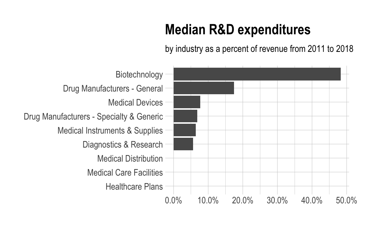
$ med_rnd_rev <dbl> 0.48317287, 0.05620271, 0.17451442, 0.06851879,…

9. Create a static bar chart.

• use ggplot to initialize the chart

• data is df

• the variable industry is mapped to the x-axis

  • reorder it based on the value of med_rnd_rev

• the variable med_rnd_rev is mapped to the y-axis

• add a bar chart using geom_col

• use scale_y_continuous to label the y-axis with percent

• use coord_flip() to flip the coordinates

• use labs to add title, subtitle and remove x and y-axis

• use theme_ipsum() from the hrbrthemes package to improve the theme

ggplot(data = df, 
  mapping = aes(
  x = reorder(industry, med_rnd_rev),
  y= med_rnd_rev
)) +
  geom_col() +
  scale_y_continuous(labels = scales::percent) +
  coord_flip() +
  labs(
    title = "Median R&D expenditures",
    subtitle = "by industry as a percent of revenue from 2011 to 2018",
    x = NULL, y = NULL) +
  theme_ipsum()

10. See the last plot to preview.png and add to the yaml chunk at the top.

ggsave(filename = "preview.png", 
       path = here::here("_posts", "2021-03-11-joining-data"))

11. Create an interactive bar chart using the package echarts4r

• start with the data df

• use arrange to reorder med_rnd_rev

• use e_charts to initialize a chart

  • the variable industry is mapped to the x-axis

• add a bar chart using e_bar with the values of med_rnd_rev

• use `e_flip_coords() to flip the coordinates

• use e_title to add the title and the subtitle

• use e_legend to remove the legends

• use e_x_axis to change format of the labels on the x-axis to percent

• use e_y_axis to remove labels on y-axis

• use e_theme to change the theme. here

df %>% 
  arrange(med_rnd_rev) %>% 
  e_charts(
    x = industry,
    ) %>% 
  e_bar(
    serie = med_rnd_rev,
    name = "median"
  ) %>% 
  e_flip_coords() %>%
  e_tooltip() %>%
  e_title(
    text = "Median industry R&D expenditures",
    subtext = "by industry as a percent of revenue from 2011 to 2018",
    left = "center") %>%
  e_legend(FALSE) %>% 
  e_x_axis(
    formatter = e_axis_formatter("percent", digits = 0)
  ) %>%
  e_y_axis(
    show = FALSE
  ) %>% 
  e_theme("sakura")